Instance Masks from Shared Features

A box around a stop sign also catches some of the trees and sky behind it. If you're building an app that selects the sign, those extra pixels matter. The pole is a little harder still. It is thin, partly hidden by the sign, and its outline changes along its length. We need a mask to describe which pixels belong to each object.

In Mirage, we build these masks from the image features already used for detection. We compute 32 spatial maps that all objects can share, then give each object 32 coefficients to combine them. That lets us reuse most of the spatial work. On the CPU, we go a step further and compute an object's coefficients from just a $5\times5$ feature patch when its mask is requested.

The shared-prototype construction comes from YOLACT. We'll follow it from image features to an outline, then look at why such a small patch is enough for the coefficients. Along the way, the geometry helps explain both what sharing saves and what it asks the model to give up.

Two branches from one image

We need both an understanding of the scene and enough local detail to follow an edge. The encoder sees a letterboxed $512\times512$ canvas, and its coarse $16\times16$ grid carries scene context. A feature pyramid brings those features together with earlier stem features at $32\times32$ and $64\times64$, producing

$D\in\mathbb R^{64\times64\times128}.$

This grid is shared with the detection head. The mask head also receives a shallower stem feature map $S_4\in\mathbb R^{128\times128\times64}$, with one cell per four canvas pixels. A learned pointwise projection and nearest-neighbour upsampling combine them,

$U=V_{128}\odot\left[\operatorname{up}_2(D)+W_eS_4\right],\qquad W_e\in\mathbb R^{128\times64}.$

$V_{128}$ marks valid image cells, excluding letterbox padding. You can think of the two terms as meeting at different scales. Upsampling carries the dense features onto a finer grid, while $S_4$ contributes detail from an earlier stage. Upsampling alone would only repeat the coarser cells.

Two separate branches then produce

$P=f_p(U)\in\mathbb R^{128\times128\times32},\qquad C=f_c(D)\in\mathbb R^{64\times64\times32}.$

$P$ contains the shared prototype maps. $C$ tells us how to combine them at each possible object centre. Writing out the full grid makes the mathematics easier to follow. Later, we'll only compute the entries an object actually needs.

Shared maps, one coefficient vector per object

stop signpole

stop sign64%

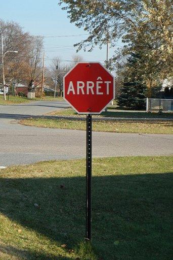
The shared maps stay the same. Selecting another object changes its coefficients and box support.

What each branch computes

Both branches have two residual blocks followed by a projection to 32 channels. They have the same shape of computation and independent weights. Writing $N_i$ for channelwise RMS normalisation with a learned scale at each location,

$f(Y^{(0)})=W_{\mathrm{out}}\operatorname{SiLU}(N_{\mathrm{out}}(Y^{(2)})).$

Each depthwise convolution mixes spatial neighbours within a channel. Each $128\times128$ pointwise matrix mixes channels within a cell. The final $32\times128$ projection has no bias or output activation.

Both prototypes and coefficients can be positive or negative. A coefficient can strengthen a pattern or subtract it from the combination. The maps are computed afresh for each image, and an individual map may contain parts of several objects. The useful shape appears when we combine them.

For an object with predicted box $b_k$, let $c_k$ be its box-centre cell on the $64\times64$ grid. Its coefficients and mask logits are

$a_k=C[c_k],\qquad \ell_k(p)=\sum_{r=1}^{32}a_{kr}P_{pr}.$

The engine evaluates the sigmoid within the box support and sets the probability to zero outside it,

$m_k(p)=\mathbf1[p\in\Omega(b_k)]\,\sigma(\ell_k(p)).$

For a very small box, no mask-grid cell centre may fall inside its edges. We include the box-centre cell in the support so that the mask still has somewhere to appear. If you're porting the head, keep this rule and the detector's coordinate rounding together. They matter most for the smallest objects.

Seeing the mask in two spaces

There are two useful ways to picture this combination. In image space, each prototype is a sheet of signed values laid over the same grid. The coefficients scale those sheets before we add them. The sign of the sum tells us which grid cells pass the default mask threshold within the box.

Now look at one mask-grid cell across all 32 sheets. Its values form a vector $P_p\in\mathbb R^{32}$. For a nonzero coefficient vector $a_k$, the equation $a_k^TP_p=0$ defines a hyperplane through the origin of this feature space. At the default threshold of $0.5$, a grid cell inside the box is selected when

$\sigma(a_k^TP_p)\ge\tfrac12\quad\Longleftrightarrow\quad a_k^TP_p\ge0.$

So the same mask is also a geometric selection of cell vectors on one side of a hyperplane. Changing the direction of $a_k$ changes which vectors it selects. The plane is flat in feature space, but the selected cells can trace a curved outline or several disconnected pieces in the image. The figure's pole is one example of a mask with separate pieces.

This is why the shared maps need to preserve useful differences between locations. If two cells have identical prototype vectors, the coefficients alone cannot separate them. Different box supports can still exclude one of them.

Flatten the spatial grid so that $P\in\mathbb R^{16384\times32}$, and stack $K$ coefficient vectors into $A\in\mathbb R^{K\times32}$. Before cropping and sigmoid, all instance logits are

$L=AP^T,\qquad \operatorname{rank}(L)\le32.$

All the logit fields for this image live in the span of the same 32 maps. We can still describe more than 32 objects by choosing different combinations and box supports. The bound tells us how much variation the shared representation can express before cropping and sigmoid. Those later operations can increase the rank of the final mask matrix.

This sharing has a cost. If the maps lose the distinction between a thin pole and its background, changing coefficients may not bring it back. The $128\times128$ grid also limits spatial detail, and a box that is too tight clips away part of the object. These are different ways a contour can go wrong, even when its name is correct.

Why a five-cell patch is enough

Now return to the coefficient grid $C$. For a particular object, we only use the vector at its box centre. To find out how much work that needs, start at that centre and trace its dependencies backwards.

Each $3\times3$ convolution expands the required neighbourhood by one cell on every side. There are two such convolutions, so a single cell grows first to a $3\times3$ square and then to a $5\times5$ square. Everything else in the branch acts within each cell. Its receptive-field width on $D$ is therefore

$R=1+(3-1)+(3-1)=5.$

To obtain $C[c_k]$, the CPU copies a $5\times5\times128$ neighbourhood centred on $c_k$, runs the branch on this patch, and keeps its central output. Padding outside the feature grid and the valid-image mask follow the same rules as the full branch.

The artificial patch boundary is too far away to affect the central output through two layers. This is the reason we can replace the full-grid calculation with a local one. It relies on every operation having the locality described above. Adding global pooling, attention or a normalisation over the whole grid would change the dependency picture.

We checked this with synthetic 128-channel features, including centres near image and padding edges where mistakes are easy to miss. The patch and full-grid outputs agreed to floating-point precision. That gives us a check of the local computation; judging the masks themselves still needs images and reference masks.

Counting padded convolution taps and excluding normalisation, activations and masking, one branch location uses

$2(9\cdot128+128^2)+128\cdot32=39{,}168$

multiply-accumulates. A full coefficient grid uses 4,096 locations. A requested patch uses 25. That is about 160.4 million multiply-accumulates for the dense map versus 0.98 million per requested object for the patch implementation. Several objects may repeat work on overlapping patches. These are operation counts for the coefficient branch, not whole-model speedups.

The prototype maps are computed on the first mask request and reused for the remaining objects in that image. Their FP32 cache occupies 2 MiB. Avoiding the dense coefficient map saves another 0.5 MiB of output storage, although patch intermediates still need memory. Image features, prototype computation, mask assembly and output conversion remain part of the cost.

From a probability field to an outline

Once we have a probability field, we still need to decide what to give the application. An outline is convenient for drawing over a camera view. A bitmap is more useful when you need to select or count individual pixels. You can choose the representation in the same call that describes the objects.

import cactus

vision = cactus.Mirage()
result = vision.describe(
    "photo.jpg",
    sections=["objects"],
    fields=["bbox", "score", "mask"],
    mask_format="polygons",
)

For polygon output, the engine traces the default probability threshold of $0.5$ using marching squares. Edge crossings are interpolated between neighbouring probabilities, then the contours are simplified. Coordinates are mapped back to the original image and expressed on axes from 0 to 1000.

The formats differ in what they retain.

For the pole in the example, polygons keeps both exterior pieces. largest keeps just the larger one, while merged draws bridges to put them in a single path. Those bridges can cross background pixels. Polygon modes also omit hole boundaries, so choose bitmap when those interior gaps matter to your application.

For the bitmap, the engine bilinearly samples the probability field onto the original image, thresholds it and clips it to the box. The result contains size in height-width order and counts beginning with a background run. It is an RLE object, not an array of pixel rows. Thresholding and interpolation do not commute, so a rasterised polygon need not match this bitmap pixel for pixel.

Where the name and score come from

The last step is attaching the contour to the object your app sees in the result. The language decoder supplies a name and attributes, along with a reference to a proposed region. That reference brings in the mask. Its coefficients were computed from image features at the box centre, independently of the words used to name it.

This places Mirage alongside several related approaches with different interfaces. Segment Anything accepts prompts such as points to select a mask. CondInst predicts parameters for a small mask network for each instance. Here, we select a proposed object and combine shared image-dependent prototypes.

When you inspect the result, read the object's score as its detection-heatmap score. The name and contour need their own checks. A confident proposal can still have an inaccurate mask or the wrong name.

Supplying the correct boxes during evaluation helps isolate the mask head. Evaluating the whole system asks more of it, because the proposals must also be found, selected and named correctly. Keeping that distinction, the mask resolution and the output format visible makes results easier to interpret and reproduce.

If you'd like to see where this division of work comes from, the structured perception article explains the broader design. OCR decoding follows the same idea for text. Try the Mirage playground with a thin object or two overlapping objects, and look at where the contour follows them and where it falls short. The same outputs are available through the Cactus package.